Welcome to another entry in our series of Dr. Wayne Winston’s best Excel tips! I’m Wayne Winston, Becker’s resident expert on all things Microsoft Excel. Let’s learn another helpful Excel skill that can make your accounting and finance work a bit easier.
As accountants, we often have to deal with unorganized data that can come from a multitude of sources.
And, when it comes time to import data into Excel from the web or a database, the data can be messy or does not come into Excel in a usable format. Luckily, the Power Query tool can be used to transform the data into a useful format. In this article, we will illustrate many of Power Query’s data transformation capabilities.
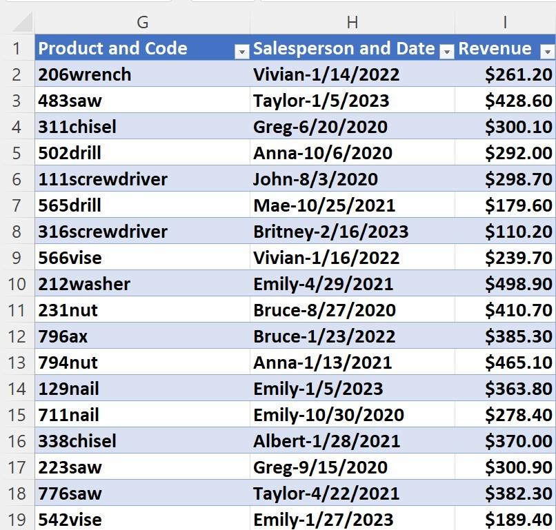
Each row of the workbook in Figure 1 (copy and paste link into a new browser tab to open) contains the following information on sales at a local hardware store:
- Product code and product sold (column G)
- Salesperson and date of transaction (column H)
- Transaction revenue (column I)
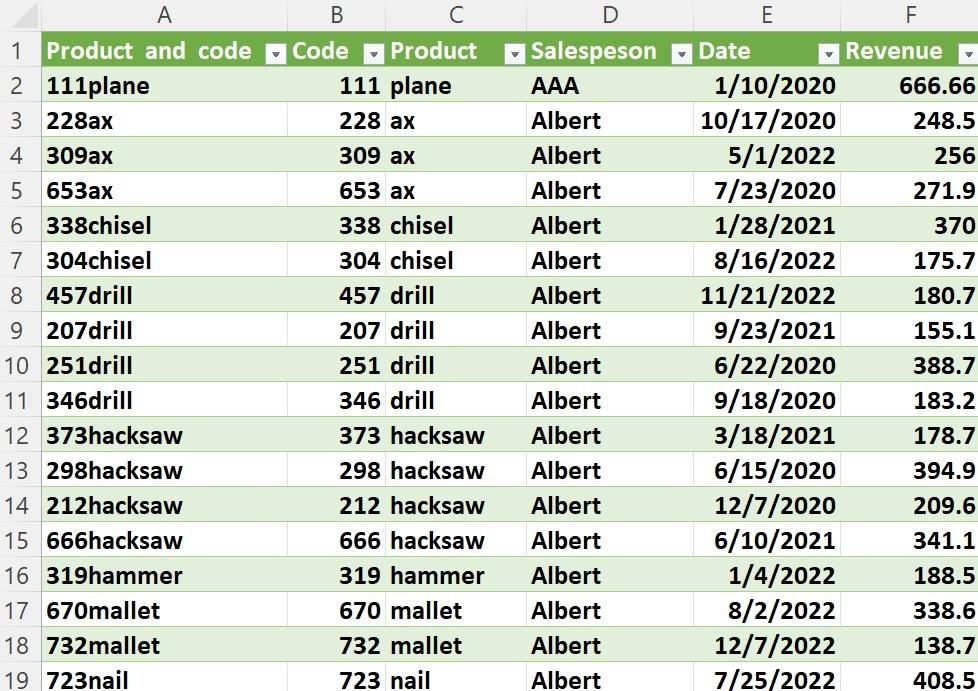
We want to use Power Query to place the information for product code, product, salesperson and date of sale in separate columns, sort transactions by salesperson, and then sort by product in A-Z order. Also, when new data is added, a simple refresh should update our results. Your result should look like Figure 2.
Figure 1: Messy hardware store data
Figure 2: “Cleaned up” data
To start, copy and paste this link for the “messy” data file, and this file for the “cleaned up” data file into new browser tabs to download the Excel workbooks and follow along.
To clean up the data, proceed as follows:
- In the “messy” data file, click into the pivot table.
- In the Data tab, in the Get &Transform Data group, click the From Table/Range or From Sheet (the name depends on how recently your Office 365 was updated) to import the data into the Power Query Editor window.
- When the Power Query Editor window opens, select the Product and Code column.
- In the Transform group of the Home tab, click the Split Column button and choose By Number of Characters from the menu that appears.
- The Split Column by Number of Characters dialog box opens. Type 3 in the Number of Characters box, and choose the Once, As Far Left as Possible, option button. Click OK.
- Right-click the heading on the first new column (or double click into the heading box). Choose Rename, and type a new name for the column - in this case, Product. Repeat this step for the second new column and name it Code.
- Select the Salesperson and Date column.
- In the Transform group of the Home tab, click the Split Column button and choose By Delimiter from the menu that appears.
- The Split Column by Delimiter dialog box opens. Open the Select or Enter Delimiter menu and choose Custom. Then, in the box that appears, enter a hyphen (-). Finally, leave the other settings at their defaults and click OK.
- Right-click the heading of the new column, choose Rename, and type a new name for the column - in this case, Salesperson. Repeat this step for the second new column to name it Date.
- Select the Salesperson column. Then, click the A-Z button in the Sort group of the Home tab. Repeat this step for the Product column.
- In the Power Query Editor window’s Home tab, click the Close & Load button in the Close group. Alternatively, open the File menu and choose Close & Load.
- Add a new row of data for a salesperson named AAA in your original sheet. In your new sheet, click Refresh All in the Data tab. Your new row of data will be properly transformed and appear as the first row of the query result.
This is our last article on Power Query. I hope I have convinced you that Power Query can automate a lot of drudgery and make you more productive in the workplace!
Want to improve your accounting Excel skillset? Enroll in Becker’s Microsoft® Excel Fundamentals + Data Analytics Certificate and learn essential Excel functions for accounting, from fundamentals all the way to in-depth applications of data analytics.
Read the first article in Dr. Wayne Winston’s Microsoft® Excel Power Query series.


